pacman::p_load(ggstatsplot, plotly, crosstalk, DT, ggdist, gganimate, FunnelPlotR, knitr, gifski, tidyverse)Take-Home_Ex03
Overview
The objective is to uncover the salient patterns of the resale prices of public housing property by residential towns and estates in Singapore by using appropriate analytical visualization techniques.
The primary focus is on 3-ROOM, 4-ROOM, and 5-ROOM types for the period 2022.
Data
Resale flat prices based on registration date from Jan-2017 onwards is used to prepare the analytical visualization. It is available at Data.gov.sg.
Data Preparation
Loading the packages
The required packages are loaded for the purpose of visualization.
Loading the data
Load the downloaded data from Data.gov.sg.
flats_data <- read_csv("data/resale-flat-prices-based-on-registration-date-from-jan-2017-onwards.csv")Filter the data
Filter the data for the year 2022 and flat type 3 Room, 4 Room, and 5 Room.
filtered_flats_data <- filter(flats_data, grepl('2022', month) & flat_type %in% c("3 ROOM", "4 ROOM","5 ROOM"))After exploring the data, it was discovered that the columns storey_range and remaining_lease requires the necessary change.
Change the order of the storey_range
Change the order of the storey_range,
storey_order <- c("01 TO 03", "04 TO 06", "07 TO 09", "10 TO 12", "13 TO 15", "16 TO 18", "19 TO 21", "22 TO 24", "25 TO 27", "28 TO 30", "31 TO 33", "34 TO 36", "37 TO 39", "40 TO 42", "43 TO 45", "46 TO 48", "49 TO 51")

updated_flat_data <- filtered_flats_data %>%
  mutate (storey_range = factor(storey_range, levels = storey_order)) %>%
  ungroup()
Change the type of remaining_lease
Change the type of remaining_lease from string to integer,
updated_flat_data$remaining_lease_int <- as.numeric(gsub("([0-9]+).*$", "\\1", filtered_flats_data$remaining_lease))Data Visualization
Now we will be exploring the data visually,
Distribution of storey_range
ggplot(data = updated_flat_data,
       aes(y = storey_range)) +
geom_bar() 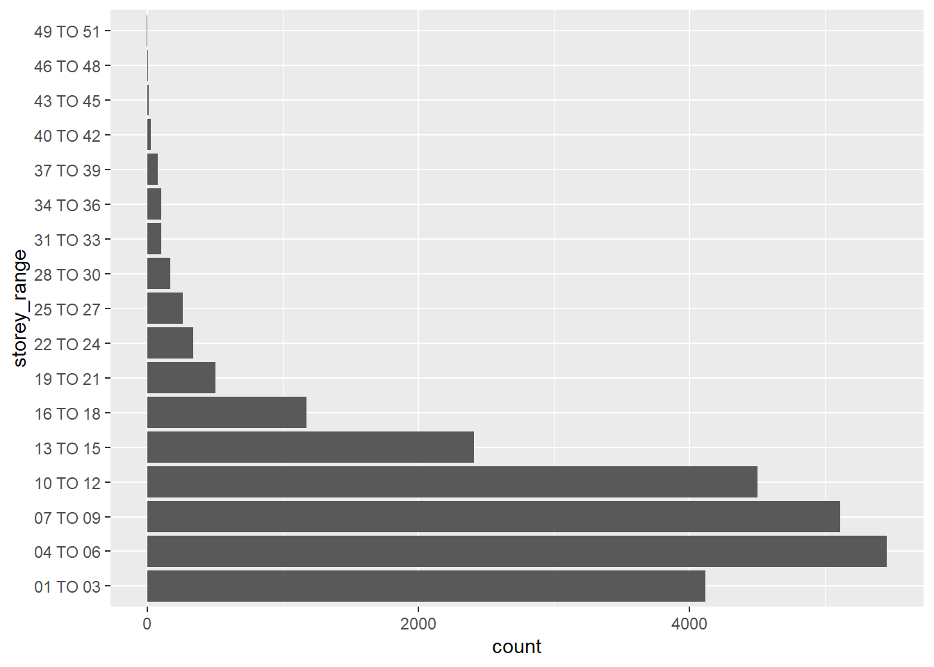
From the above graph, it can be observed that storey_range from 01 TO 30 have the majority of the flats in Singapore, 2022.
One-way ANOVA flat_type and resale_price
ggbetweenstats(
  data = updated_flat_data,
  x = flat_type,
  y = resale_price,
  type = "p",
  mean.ci = TRUE,
  pairwise.comparisons = TRUE,
  pairwise.display = "s",
  p.adjust.method = "fdr",
  messages = FALSE
)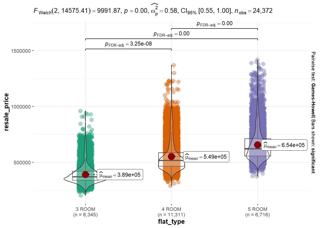
From performing the one-way ANOVA test between flat_type and resale_price, the p-value(<0.05) suggests that the mean value of various flat_type is different from one another.
H0: Mean resale_price values of different flat_type are equal to one another.
H1: Mean resale_price values of different flat_type are unequal.
Visualizing uncertainty with Hypothetical Outcome Plots(HOPs)
devtools::install_github("wilkelab/ungeviz")library(ungeviz)
filtered_sr_flats_data <- filter(updated_flat_data, storey_range %in% c("43 TO 45"))ggplot(data = filtered_sr_flats_data,
(aes(x = factor(flat_type), y = resale_price))) +
geom_point(position = position_jitter(
width = 0.05),
color = "#0072B2", alpha = 1/2) +
geom_hpline(data = sampler(25, group = flat_type), color = "#D55E00") +
theme_bw() +
# `.draw` is a generated column indicating the sample draw
transition_states(.draw, 1, 3)
To furthermore analyse the data individually for different, lets find the unique number of different categorical values in the dataset.
unique(updated_flat_data$town) [1] "ANG MO KIO" "BEDOK" "BISHAN" "BUKIT BATOK"
[5] "BUKIT MERAH" "BUKIT PANJANG" "BUKIT TIMAH" "CENTRAL AREA"
[9] "CHOA CHU KANG" "CLEMENTI" "GEYLANG" "HOUGANG"
[13] "JURONG EAST" "JURONG WEST" "KALLANG/WHAMPOA" "MARINE PARADE"
[17] "PASIR RIS" "PUNGGOL" "QUEENSTOWN" "SEMBAWANG"
[21] "SENGKANG" "SERANGOON" "TAMPINES" "TOA PAYOH"
[25] "WOODLANDS" "YISHUN" unique(updated_flat_data$flat_model) [1] "New Generation" "Improved" "Model A"
[4] "DBSS" "Simplified" "Premium Apartment"
[7] "Standard" "Model A-Maisonette" "Model A2"
[10] "Type S1" "Type S2" "Premium Apartment Loft"
[13] "Adjoined flat" "Terrace" "3Gen"
[16] "Improved-Maisonette" unique(updated_flat_data$floor_area_sqm) [1] 73.0 67.0 68.0 82.0 83.0 75.0 74.0 60.0 81.0 92.0 99.0 93.0
[13] 98.0 100.0 91.0 106.0 90.0 85.0 119.0 120.0 118.0 125.0 110.0 112.0
[25] 69.0 59.0 70.0 66.0 65.0 88.0 94.0 95.0 87.0 104.0 103.0 107.0
[37] 84.0 105.0 108.0 123.0 122.0 121.0 139.0 115.0 133.0 113.0 126.0 64.0
[49] 116.0 114.0 111.0 130.0 77.0 102.0 117.0 101.0 96.0 149.0 62.0 63.0
[61] 80.0 132.0 89.0 128.0 97.0 138.0 79.0 109.0 124.0 127.0 134.0 131.0
[73] 57.0 56.0 61.0 52.0 72.0 58.0 129.0 136.0 140.0 53.0 76.0 86.0
[85] 71.0 137.0 135.0 150.0 60.3 78.0 54.0 142.0 55.0 159.0 141.0 154.0
[97] 63.1 144.0 155.0 157.0 51.0 152.0 143.0One-way ANOVA flat_type and floor_area_sqm
ggbetweenstats(
  data = updated_flat_data,
  x = flat_type,
  y = floor_area_sqm,
  type = "p",
  mean.ci = TRUE,
  pairwise.comparisons = TRUE,
  pairwise.display = "s",
  p.adjust.method = "fdr",
  messages = FALSE
)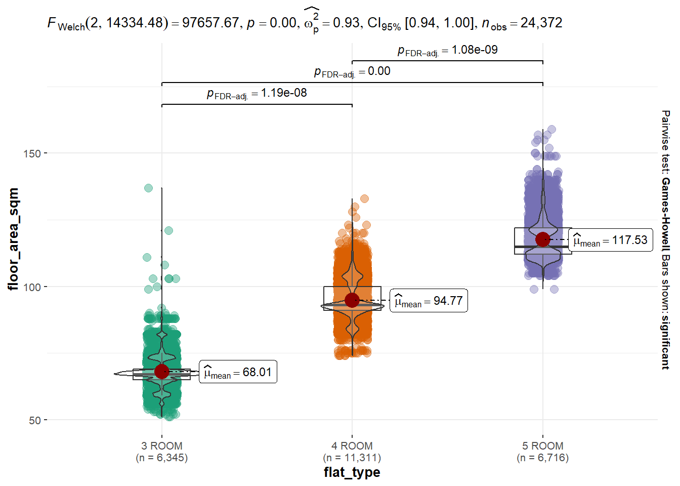
From performing the one-way ANOVA test between flat_type and floor_area_sqm, the p-value(<0.05) suggests that the mean value of various flat_type is different from one another.
H0: Mean floor_area_sqm values of different flat_type are equal to one another.
H1: Mean floor_area_sqm values of different flat_type are unequal.